InstrumentQC_Path <- file.path("C:", "Users", "JohnDoe", "Documents", "InstrumentQC")

InstrumentQC_Path
[1] "C:/Users/JohnDoe/Documents/InstrumentQC"As mentioned in the introduction, within the .R and .qmd files are lines of code corresponding to file.paths. These act like addresses that the code uses to find the correct folders that contain daily QC .fcs and .csv files on your individual computer. Since where SpectroFlo (and its associated files) is on your computer may be different from that of our instruments computers, you will need to update these file paths to allow your computer to retrieve the daily QC files from the correct folder when the R scripts are run.
Let’s start by working with the example of our InstrumentQC repository. On our Windows computer, it is located in our Documents folder. This folder itself is located within an individual users folder located on the computers “C:” drive.
Consequently, when we provide the file.path to R, we need to provide all these parent folders When we provide a file.path to R, we need to account for all these parent folders when assembling a filepath.
Now, let’s examine the contents of this folder:
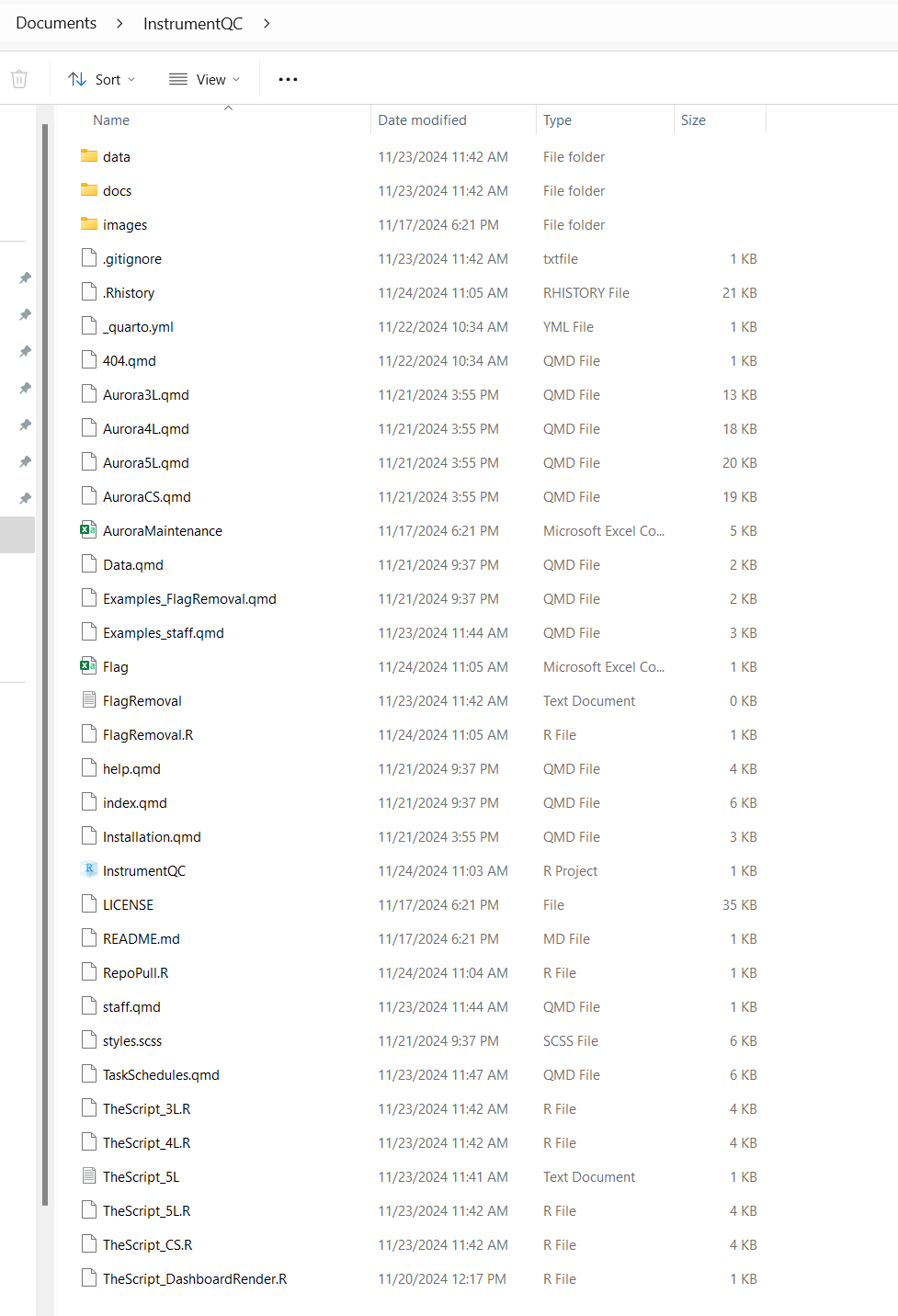
As we mentioned in Pieces of a Bigger Picture, this folder contains the Instrument.R files that run the code that processes the newly acquired QC data, as well as the Instrument.qmd files that create the individual instrument webpages. Consequently, in Data Transfer section when we need to edit the file paths to these scripts, we would provide a file.path that resembles the following:
ThisIsTheRFileYouAreLookingFor <- file.path("C:", "Users", "JohnDoe", "Documents", "InstrumentQC", "TheScript_3L.R")
ThisIsTheRFileYouAreLookingFor
[1] "C:/Users/JohnDoe/Documents/InstrumentQC/TheScript_3L.R"Alternatively, we can reuse the file.path that we had just corresponding to the InstrumentQC folder location stored in the InstrumentQC_Path we ran in the last example, and use it to shorten the number of folders we need to type:
If you are building a website containing multiple instruments, you will be needing the file.path locations to each instruments data folder to be able to retrieve the data for plotting. Let’s go ahead and double click on data and see the contents.
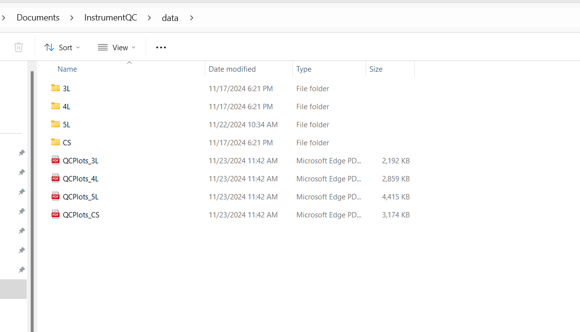
As you can see, here are the individual folders.
Within the Instrument.qmd files, there is a file.path expression that resembles the following code chunk:
In this case, the file.path for InstrumentQC_Path first gets extended to include the data folder in the variable MainFolder. Then, the instrument folder for the instrument of listed gets designated by the variable TheList. Consequently, when MainFolder and TheList are passed to the DailyQCParse and QCBeadParse functions (that process the individual .fcs and .csv files) they know which insturment folder to copy the newly acquired data to (vs. the other instrument folders)
[1] "C:/Users/JohnDoe/Documents/InstrumentQC/data/5L"If we go ahead and click on the individual instrument folder, we see that it is currently empty outside of the Archive folder.
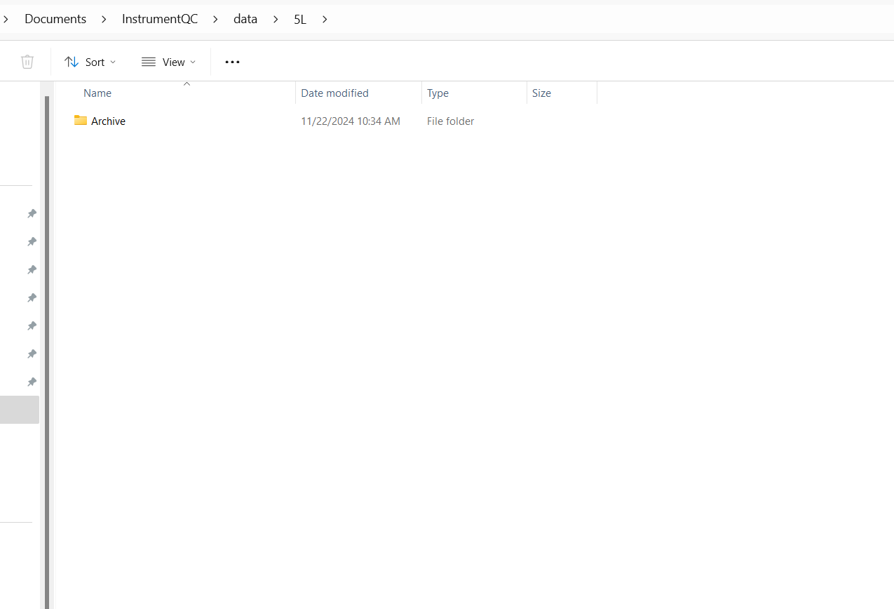
If we were to check it in the middle of the processing of the newly acquired QC data, we would see the newly acquired .fcs and .csv files copied to this folder waiting to be processed and added to the .csv files that we can find within the Archive folder. After successfully being added to the archive, these copied files are deleted, leaving the folder empty.
Checking within Archive, we can see two folders:
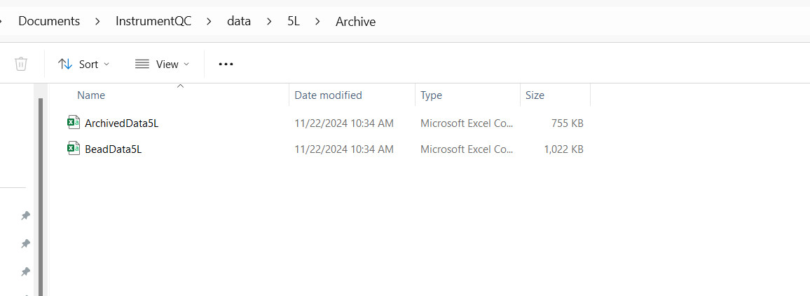
For Cytek Instruments, data derriving from the DailyQC.csv files is processed and stored as the ArchivedData.csv. For data derrived from processed before/after QC bead .fcs files, these are stored in the BeadData.csv. For the BD instruments, everything is currently derrived from CST bead .fcs files, consequently stored in the HolisticData.csv file.
It is from these instrument specific archive .csv files that all the plots found in the individual instrument webpages get generated, so knowing the file.paths to these individual .csv files in important to have ready to swap in!
To recap, for all instruments, you will need to have the file.path to the InstrumentQC folder. For the individual instruments, you will need to provide to their Instrument.R processing script the path to the Instrument folder where the newly acquired data will be transferred to before processing. And finally, when modifying the Instrument.qmd files to generate plots of the archive data, you will need the file.paths for the individual Archive.csv files for their respective data types.
Now that we have an initial understanding of file.paths, it is time to go find the file.paths to where the newly acquired QC data is being stored. Once we have identified these file.paths, we can provide them to the Instrument.R script to allow it to copy these files to the location designated by the Instrument Folder file path we identified above.
We will for now focus on finding the locating the SpectroFlo .fcs and .csv files. The process of finding the .fcs files acquired on our BD instruments is similar, but generally, we are storing those .fcs files in a specific folder of our own creation (rather than the software storing in a designated location).
The SpectroFlo-associated folders that contain QC data can be found in “CytekbioExport” folder. Depending on your individual installation selections, the location of this folder may vary. For most of our instruments, it can be found in the “C:” drive.
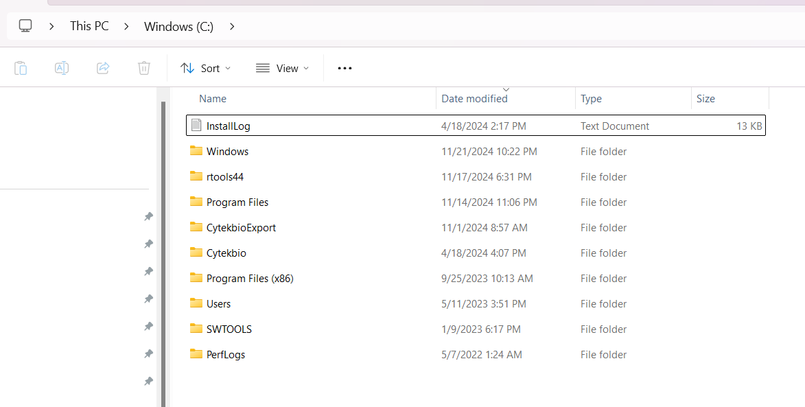
If you are ever uncertain about a folder location, right click the > symbol and select copy address as text. Paste the location into your terminal and copy the relevant folder names into your file.path() argument.
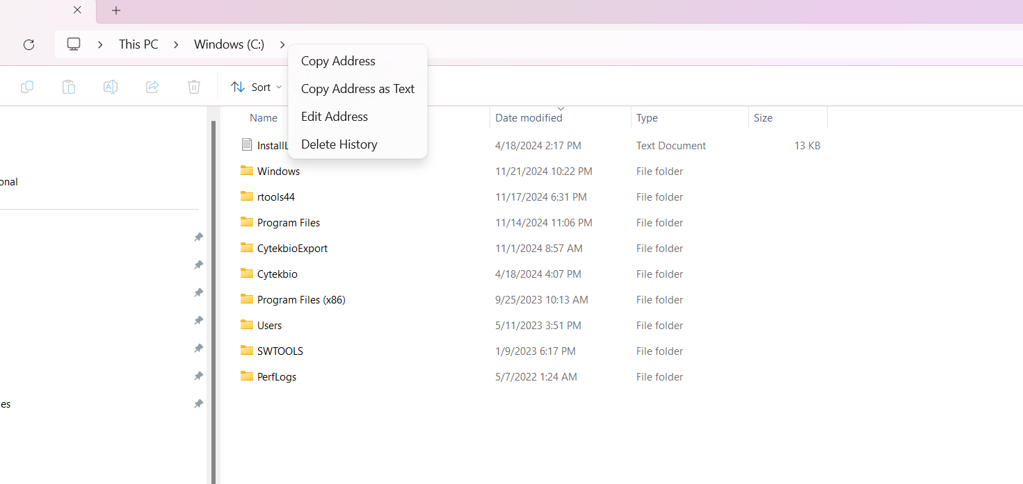
When we paste in this manner, we get something like this: C:\Cytekbio. For file.paths, both “/” and “"” designate a descending hierarchy going from parent folders to the folder/file of interest. Unfortunately, which is used depends on what operating system your computer is running on (Windows, Mac or Linux).
One of the reasons I recommend building your filepaths with file.path() is that it is operating system agnostic. Additionally, R makes you switch Windows right-click copy file.paths from \ be switched to / before it will recognize them. onsequently, building with the file.path() function is easier in the long run than remembering if its the / or slash that causes issues with R in Windows.
So to build the file.path to Cytekbio Export, we would write something like the following:
[1] "C:/CytekbioExport"Let’s go ahead and double click and see what is inside the folder:
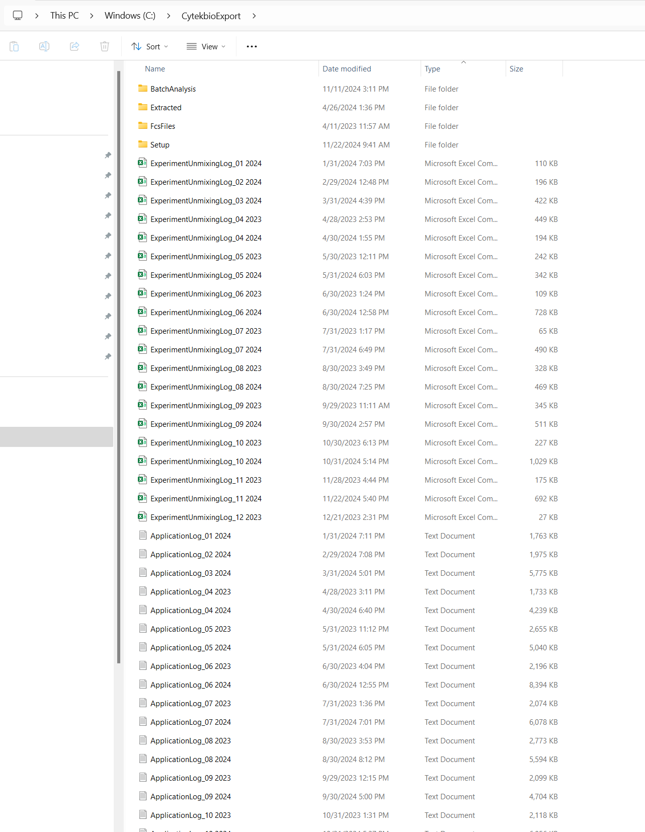
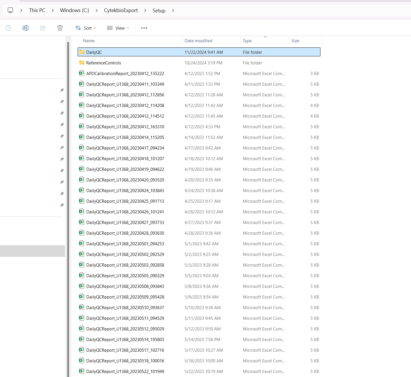
We can see in this case that we have folders for Experiments, FCSFiles and Setup. We additionally see files corresponding to the ApplicationLog, SetupEngineLog, AppLoginLog and ExperimentUnmixingLog that track various activity previously carried out in SpectroFlo.
Let’s navigate into the folder “Setup”
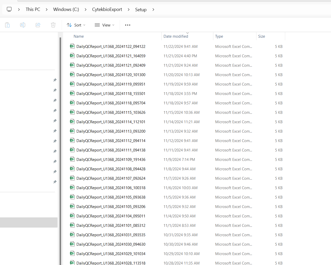
The file.path for this location would resemble the following:
[1] "C:/CytekbioExport/Setup"It is within this folder that the DailyQC reports are stored as .csv files. Opening them, we can see they contain a lot of the same data we can see in the Daily report. Explanation of the individual elements is beyond the scope of this current tutorial, but the majority of this data gets extracted and utilized for the dashboard in various ways for the Gain and RCV plots.
Unfortunately, these .csv does not follow a “tidy” format (having gaps in spaces and rows rather than equally filled rectangular space). Consequently, a bunch of functions in the Luciernaga R package are used to process the data behind the scenes until it is returned in a “tidy” format that R can work with (these can later be downloaded from the Data tab on the dashboard).
This file.path (SetupFolderPath) is the one we will need to provide to the Instrument.R file so that it knows where to find the new DailyQC.csv files to allow them to be copied to the respective InstrumentQC Instrument Folder for further processing. Make a note of this file path before continuing.
In SpectroFlo, Daily QC produces a single .fcs file that can be processed to monitor changes in MFI. These .fcs files can be found within the Setup folder inside the DailyQC folder.
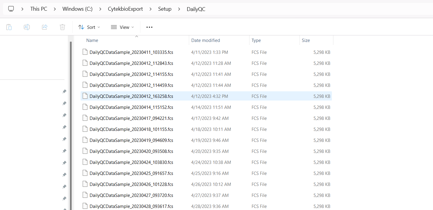
Therefore, to use them, we would need to modify the file.path to include this additional folder when modifying the Instrument.R script to find the .fcs files.
For our institution, separate from the SpectroFlo DailyQC .fcs files, we acquire 3000 events of the same QC beads before and after running DailyQC to provide additional information about the changes in MFI resulting from DailyQC.
These are acquired within a SpectroFlo under either the Admin or Core account, in a single experiment for a given month, which the before and after .fcs files organized as individual tubes. Consequently, these .fcs files are stored in the same folder where other users experiments and data are also stored before they are exported as zipped folders. At our core, due to lack of memory space on the C: drive, these folders can be found on a large external hard drive.
Consequently, if we want to provide these files to R for processing, we need to adjust the file.path, and provide a mechanism to identify the folder based on the given month/day.
Let’s start looking in the External Hard Drive and build out the file.path:
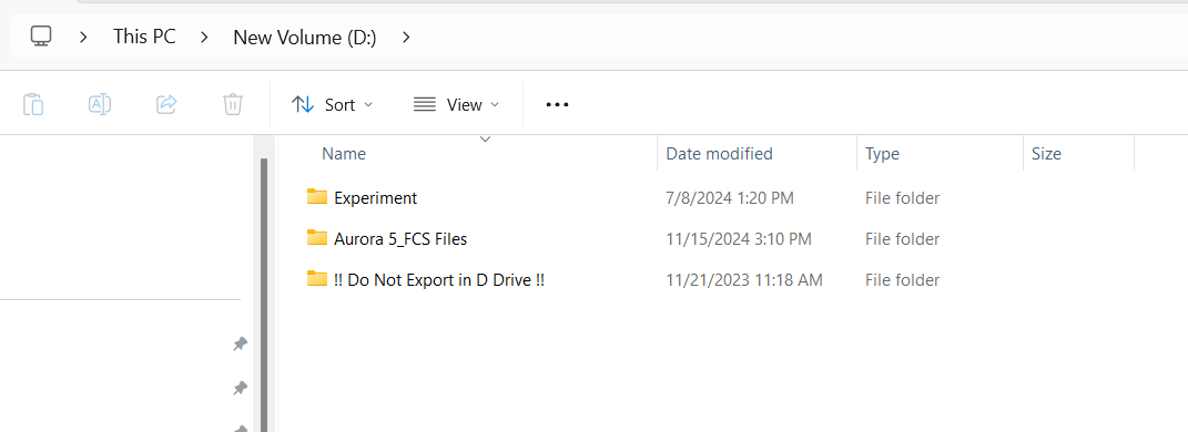

[1] "D:/Aurora 5 FCS_Files/Experiments"At this point, we are in the experiments folder and can see the folders for all the respective users. Since the Admin account was used for this instrument for the acquisition of the before/after QC .fcs files, let’s navigate into this folder:

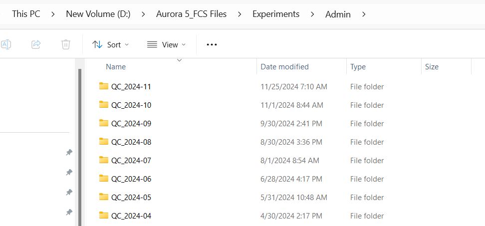
As you can see, these folders correspond to the individual experiment file names. We take care in making sure they are named consistently to allow for the Instrument.R script to recognize the correct folder containing that months data from the file name.
For example, let’s say its currently November of 2024. The Instrument.R script will need to identify this folder and check inside for newly acquired .fcs files for the given day. Within the code, the function System.time gets called to return the date and time.
From this information, we can break down the return value into Month, Date, and Time. In a simplified example, this can be used to generate the folder name, that can then be added to the file.path allowing the Rscript to find the correct folder for that given month.
Year <- lubridate::year(CurrentTime)
Month <- lubridate::month(CurrentTime)
Day <- lubridate::day(CurrentTime)

ThisFolder <- paste0("QC_", Year, "-0", Month)
ThisFolder
[1] "QC_2025-02"[1] "D:/Aurora 5 FCS_Files/Experiments/Admin/QC_2025-02"While simplified (actual code handles exceptions) you can see how a misnamed experiment name could break the Instrument.R script from finding the correct folder, let’s say for example the scrupt was looking for “QC_2024-04” but instead the experiment is saved as “QC 2020 04”. It would look for that folder, not find anything, and therefore, not copy any fcs files over to the InstrumentQC Instrument folder for processing.
This is a good thing to be aware of generally, and adjust the code as necessary to match the structure of your experiment folder names.
We have now discussed file.paths extensively, and have identified the main filepaths to important folders we will need to have to modify the various Instrument.R, Instrument.qmd, and eventually the automated task schedules. We will edit the main ones in the next article, and hopefully process your existing data into an Archive .csv file that you can start using.