Data Visualization
David Rach
University of Maryland, Baltimoredrach@som.umaryland.edu
1 June 2025
Source:vignettes/DataVisualization.Rmd
DataVisualization.RmdAbstract
Spectral Flow Cytometry (SFC) capacity to rapidly acquire large number of cellular events is similar to that of conventional flow cytometry (CFC), but it’s ability to resolve very similar fluorophores allows for marker profiling comparable to mass cytometry (MC). Unmixing controls (both single color and unstained) are critical to this process. Luciernaga is a collection of tools to enable individual users to profile quality of their unmixing controls, how they vary across experiments, and their subsequent effects on unmixing of full-stained samples.
Introduction
Spectral flow cytometry (SFC) ability to resolve the presence and relative abundance of highly similar fluorophores on individual cells is heavily dependent on the quality of the reference unmixing controls (both single-color (SC) and unstained (UC)).
Despite their critical role, there are few resources and tools (either open-source or commercial) available to evaluate the quality of the unmixing controls. This leads to individual users only becoming aware of issues after unmixing the full-stained sample when the unmixed sample looks “off”. They are subsequently left to interpret the tea leaves of their unmixed data, attempting to parse what may have led to the outcome.
Given that unmixing issues can arise from a variety of sources (multiple autofluorescences, tandem degradation, or instrumental error) that similarly can result in loss of resolution, having a way to screen for problematic unmixing controls quickly and evaluate their potential effect on re-unmixing would be useful. Additionally, tools made for these purposes can be utilized to further query how individual fluorescent signatures and brightness impact the unmixing process.
Luciernaga is an R package that attempts to address these gaps. It provides functionality to implement and tailor quality control checks of unmixing controls, characterize normalized signatures present, and evaluate their effect on unmixing. Using functional programming, it can enable data exploration and visualization for an entire data set.
These work at the individual experiment basis, but can also be combined to visualize changes in fluorescence across an experimental run to identify trends affecting single color quality. Our goal is to provide tools that others can use to further develop quantitative methods to monitor their own individual panels and instrumental configurations. We additionally leverage functional programming ability of the purrr to enable data visualization of all markers present with the resulting unmixed samples, as well as all samples present within a GatingSet at a desired gating node.
Luciernaga is a free and open source software project started at the University of Maryland, Baltimore and is under active development. It was originally designed to address issues around our cytometry core’s Cytek Aurora instruments. We would love your feedback. If you identify any bugs, please open an issue on the github repository. If you have suggestions or would like to participate in extending the functionality to other spectral cytometry instruments, please reach out to the email listed in the description.
Setup
Installing Luciernaga
We are in the process of preparing Luciernaga for submission to Bioconductor later this year. Until then, it is available for download via our GitHub.
if(!require("remotes")) {install.packages("remotes")}

if(!require("Luciernaga")){
  remotes::install_github("https://github.com/DavidRach/Luciernaga")
}

# install.packages("BiocManager")
# BiocManager::install("Luciernaga")
Loading Libraries
Luciernaga works using infrastructure provided by other Bioconductor cytometry packages. It also makes use of tidyverse packages available via CRAN to facilitate use by target audience of novice-intermediate R users. It is important to make sure that these are installed on your computer and then that the libraries are loaded.
Locating .fcs files
To get started, you will first need to provide the location on your computer where the .fcs files of interest are being stored. An example of how the author does this on their computer is provided below and can be modified for your own user and desired computer folder.
File_Location <- file.path("C:", "Users", "JohnDoe", "Desktop",
                           "TodaysExperiment")
FCS_Pattern <- ".fcs$"
FCS_Files <- list.files(path = File_Location, pattern = FCS_Pattern,
                        full.names = TRUE, recursive = FALSE)
For this vignette, we will using down-sampled .fcs files that can be found in Luciernaga’s extdata folder for our example. From the original .fcs files, we have retained 10000 events for cell unmixing controls, and 3000 for bead unmixing controls.
File_Location <- system.file("extdata", package = "Luciernaga")
FCS_Pattern <- ".fcs$"
FCS_Files <- list.files(path = File_Location, pattern = FCS_Pattern,
                        full.names = TRUE, recursive = FALSE)
head(FCS_Files[20:30], 5)
#> [1] "C:/Users/12692/AppData/Local/R/win-library/4.4/Luciernaga/extdata/CCR7_BV650(Beads).fcs"
#> [2] "C:/Users/12692/AppData/Local/R/win-library/4.4/Luciernaga/extdata/CCR7_BV650(Cells).fcs"
#> [3] "C:/Users/12692/AppData/Local/R/win-library/4.4/Luciernaga/extdata/CD107a_APC-R700(Beads).fcs"
#> [4] "C:/Users/12692/AppData/Local/R/win-library/4.4/Luciernaga/extdata/CD107a_APC-R700(Cells).fcs"
#> [5] "C:/Users/12692/AppData/Local/R/win-library/4.4/Luciernaga/extdata/CD127_BV421(Beads).fcs"
Within the extdata folder we have a mix of different files intended for different vignettes. The majority of the contents are unmixing controls and full-stained samples acquired in the process of processing a 29-color SFC panel of Cord (CBMC) and Peripheral Blood Mononuclear Cells (PBMCs), both raw and unmixed files. Additionally, there are samples that correspond to Cytek Aurora QC beads that were collected before and after the daily QC bead for instrument monitoring.
For this initial example, lets filter the list by keywords in the file name to organize them for subsequent use elsewhere in the vignette. For now, let’s subset the desired files as shown below:
QCBeads <- FCS_Files[grep("After|Before", FCS_Files)]

Unmixed_FullStained <- FCS_Files[grep("Unmixed", FCS_Files)]

Raw_FullStained <- FCS_Files[-grep(
  "Cells|Beads|Unmixed|Unstained|After|Before", FCS_Files)]

UnstainedFCSFiles <- FCS_Files[grep("Unstained", FCS_Files)]
UnstainedBeads <- UnstainedFCSFiles[grep("Beads", UnstainedFCSFiles)]
UnstainedCells <- UnstainedFCSFiles[-grep("Beads", UnstainedFCSFiles)]

BeadFCSFiles <- FCS_Files[grep("Beads", FCS_Files)]
BeadSingleColors <- BeadFCSFiles[-grep("Unstained", BeadFCSFiles)]

CellSingleColors <- FCS_Files[grep("Cells", FCS_Files)]
head(CellSingleColors, 5)
#> [1] "C:/Users/12692/AppData/Local/R/win-library/4.4/Luciernaga/extdata/CCR4_BUV615(Cells).fcs"
#> [2] "C:/Users/12692/AppData/Local/R/win-library/4.4/Luciernaga/extdata/CCR6_BV786(Cells).fcs"
#> [3] "C:/Users/12692/AppData/Local/R/win-library/4.4/Luciernaga/extdata/CCR7_BV650(Cells).fcs"
#> [4] "C:/Users/12692/AppData/Local/R/win-library/4.4/Luciernaga/extdata/CD107a_APC-R700(Cells).fcs"
#> [5] "C:/Users/12692/AppData/Local/R/win-library/4.4/Luciernaga/extdata/CD127_BV421(Cells).fcs"
Creating a GatingSet
Once we have the list of desired .fcs files, we can use the flowWorkspace to bring these individual .fcs files first into a CytoSet object, then into a GatingSet object that we can add gates to:
MyCytoSet <- load_cytoset_from_fcs(UnstainedCells, truncate_max_range = FALSE,
                                   transformation = FALSE)
#MyCytoSet
MyGatingSet <- GatingSet(MyCytoSet)
MyGatingSet
#> A GatingSet with 18 samples
For this example, we will use the openCyto package to automatically gate each of our .fcs files for the lymphocyte population. To do this, we first read in the example .csv file containing our desired gates (that can be found in Luciernaga’s extdata folder) using the data.table package
FileLocation <- system.file("extdata", package = "Luciernaga")
MyGates <- fread(file.path(path = FileLocation, pattern = 'Gates.csv'))
gt(MyGates)| alias | pop | parent | dims | gating_method | gating_args | collapseDataForGating | groupBy | preprocessing_method | preprocessing_args |
|---|---|---|---|---|---|---|---|---|---|
| singletsFSC | + | root | FSC-A,FSC-H | singletGate | FALSE | NA | NA | NA | |
| singletsSSC | + | singletsFSC | SSC-A,SSC-H | singletGate | FALSE | NA | NA | NA | |
| singletsSSCB | + | singletsSSC | SSC-A,SSC-B-A | singletGate | FALSE | NA | NA | NA | |
| nonDebris | + | singletsSSCB | FSC-A | gate_mindensity | FALSE | NA | NA | NA | |
| lymphocytes | + | nonDebris | FSC-A, SSC-A | flowClust | K=2, target=c(1e5, 5e4) | FALSE | NA | NA | NA |
For your own experiments, individual gates can be added, removed or modified to match the requirements of your own .fcs files, for additional details, please refer to the openCyto packages vignettes. Alternatively, GatingSet objects can be brought directly from several commercial software formats using the CytoML package.
Now that we have the gating information from the .csv file, we can convert them into a GatingTemplate, and append them to the .fcs files contained within the GatingSet
MyGatingTemplate <- gatingTemplate(MyGates)
gt_gating(MyGatingTemplate, MyGatingSet)
MyGatingSet[[1]]
#> Sample:  INF071_Ctrl_Unstained.fcs
#> GatingHierarchy with  6  gates
Visualizing Gates
Utility_GatingPlots
We can visualize our applied gates on their individual .fcs files
using Luciernaga’s Utility_GatingPlots() function. We can
do this individually, or iterate over the entire GatingSet using the
purrr
purrr::map() function.
To do this, we reference the data.table
imported gating information (MyGates) showcased above, and the GatingSet
object. Utility_GatingPlots() argument export = FALSE will
return a patchwork
grouped ggplot objects, return = TRUE returns the same output in a .pdf
file to the designated output location.
removestrings <-  c("DR_", "Cells", ".fcs", "-", " ")
StorageLocation <- file.path("C:", "Users", "JohnDoe", "Desktop")

IndividualPlot <- Utility_GatingPlots(x=MyGatingSet[[2]], sample.name = "GUID",
                                      removestrings = removestrings,
                                      gtFile = MyGates, DesiredGates = NULL,
                                      outpath = StorageLocation,
                                      returnType="patchwork")

IteratedPlots <- map(.x = MyGatingSet[1:3], .f = Utility_GatingPlots,
                     sample.name = "GUID", removestrings = removestrings,
                     gtFile = MyGates, DesiredGates = NULL,
                     outpath = StorageLocation, returnType="patchwork")
#> $`1`
#>
#> $`2`
Utility_IterativeGating
In the absence of an existing gating template, the
Utility_IterativeGating() function can be used to visualize
individual gate placements for specimens found in a GatingSet object. To
figure out the necessary information, we can use flowWorkspace
flowWorkspace::plot() and
flowWorkspace::gs_pop_get_gate() to find out the gate, and
the respective X and Y parameters.
plot(MyGatingSet)
gs_pop_get_gate(MyGatingSet[1], "lymphocytes")
#> $INF071_Ctrl_Unstained.fcs
#> Ellipsoid gate 'lymphocytes' in dimensions FSC-A and SSC-A

SingleSpecimen <- Utility_IterativeGating(x=MyGatingSet[1], sample.name = "GUID",
                                          removestrings = removestrings,
                                          subset = "nonDebris",
                                          gate = "lymphocytes",
                                          xValue = "FSC-A", yValue = "SSC-A",
                                          bins = 270)


AllSpecimens <- Utility_IterativeGating(x=MyGatingSet[1:3], sample.name = "GUID",
                                        removestrings = removestrings,
                                        subset = "nonDebris", gate = "lymphocytes",
                                        xValue = "FSC-A", yValue = "SSC-A", bins = 270)
#> [[1]]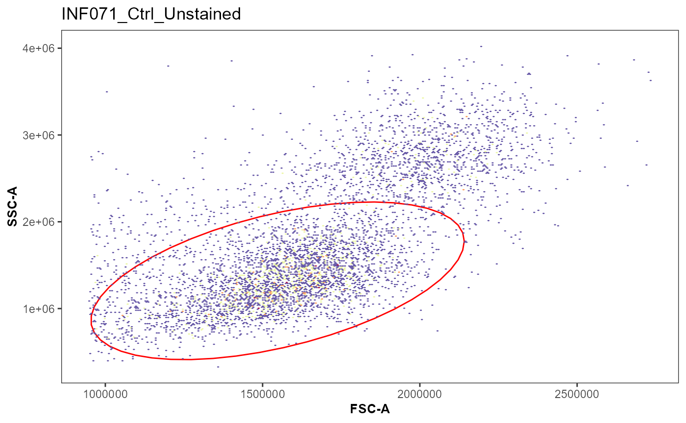
Utility_Patchwork
The previous example returned AllSpecimens, which is a list of ggplot
objects. This allows us to showcase Utility_Patchwork(). It
is a wrapper for patchwork
that is used in the background by Luciernaga’s data visualization
functions when generating .pdf files from existing ggplot objects.
Utility_Patchwork() will take the list of ggplot
objects, arrange them based on the specified number of columns and rows
into individual pages of designated width and height, and when
returntype = “pdf” save them to the designated outfolder file.path with
the desired file.name.
StorageLocation <- file.path("C:", "Users", "JohnDoe", "Desktop")

Utility_Patchwork(AllSpecimens, "LymphocyteGates", outfolder=StorageLocation,
                  thecolumns=2, therows=2, width = 7, height = 9,
                  returntype="patchwork")
#> $`1`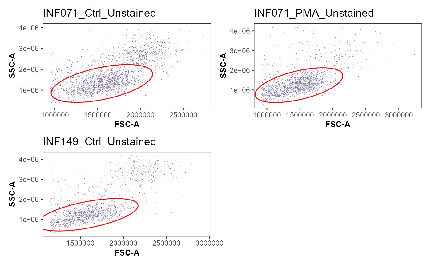
Creating a GatingSet for Unmixed .fcs files
The next couple functions are designed primarily for use with unmixed full-stained samples. We will return to the earlier example and select the corresponding example .fcs files found within Luciernaga’s extdata folder and bring them into a GatingSet object.
UnmixedFCSFiles <- Unmixed_FullStained[c(1:4)]
UnmixedFCSFiles
#> [1] "C:/Users/12692/AppData/Local/R/win-library/4.4/Luciernaga/extdata/INF071_Ctrl_Tetramer_Unmixed.fcs"
#> [2] "C:/Users/12692/AppData/Local/R/win-library/4.4/Luciernaga/extdata/INF149_Ctrl_Tetramer_Unmixed.fcs"
#> [3] "C:/Users/12692/AppData/Local/R/win-library/4.4/Luciernaga/extdata/INF179_Ctrl_Tetramer_Unmixed.fcs"
#> [4] "C:/Users/12692/AppData/Local/R/win-library/4.4/Luciernaga/extdata/ND050_15_Ctrl_Tetramer_Unmixed.fcs"
UnmixedCytoSet <- load_cytoset_from_fcs(UnmixedFCSFiles,
                                        truncate_max_range = FALSE,
                                        transform = FALSE)

UnmixedGatingSet <- GatingSet(UnmixedCytoSet)
UnmixedGatingSet
#> A GatingSet with 4 samples
Now that they are in a GatingSet object, we will identify
markers/fluorophores present for the .fcs file, and remove from the list
markers that don’t need to be transformed (example FSC, SSC, etc). We
will then bi-exponentially transform the data using flowWorkspace
flowWorkspace::flowjo_biexp_trans() before applying a
gating template.
Markers <- colnames(UnmixedCytoSet)
KeptMarkers <- Markers[-grep(
  "Time|FS|SC|SS|Original|-W$|-H$|AF", Markers)]

MyBiexponentialTransform <- flowjo_biexp_trans(channelRange = 256,
                                               maxValue = 1000000,
                                               pos = 4.5, neg = 0,
                                               widthBasis = -1000)

TransformList <- transformerList(KeptMarkers, MyBiexponentialTransform)
UnmixedGatingSet <- transform(UnmixedGatingSet, TransformList)

FileLocation <- system.file("extdata", package = "Luciernaga")
UnmixedGates <- fread(file.path(path = FileLocation,
                                pattern = 'GatesUnmixed.csv'))
UnmixedGating <- gatingTemplate(UnmixedGates)
gt_gating(UnmixedGating, UnmixedGatingSet)
UnmixedGatingSet[[4]]
#> Sample:  ND050_15_Ctrl_Tetramer_Unmixed.fcs
#> GatingHierarchy with  7  gates
And to verify successfully gated as we expected:
plot(UnmixedGatingSet)
StorageLocation <- file.path("C:", "Users", "JohnDoe", "Desktop")
removestrings <- ".fcs"

UnmixedIndividualPlot <- Utility_GatingPlots(x=UnmixedGatingSet[[2]],
                                             sample.name = "GUID",
                                             removestrings = removestrings,
                                             gtFile = UnmixedGates,
                                             DesiredGates = NULL,
                                             outpath = StorageLocation,
                                             returnType="patchwork")
#> $`1`
#>
#> $`2`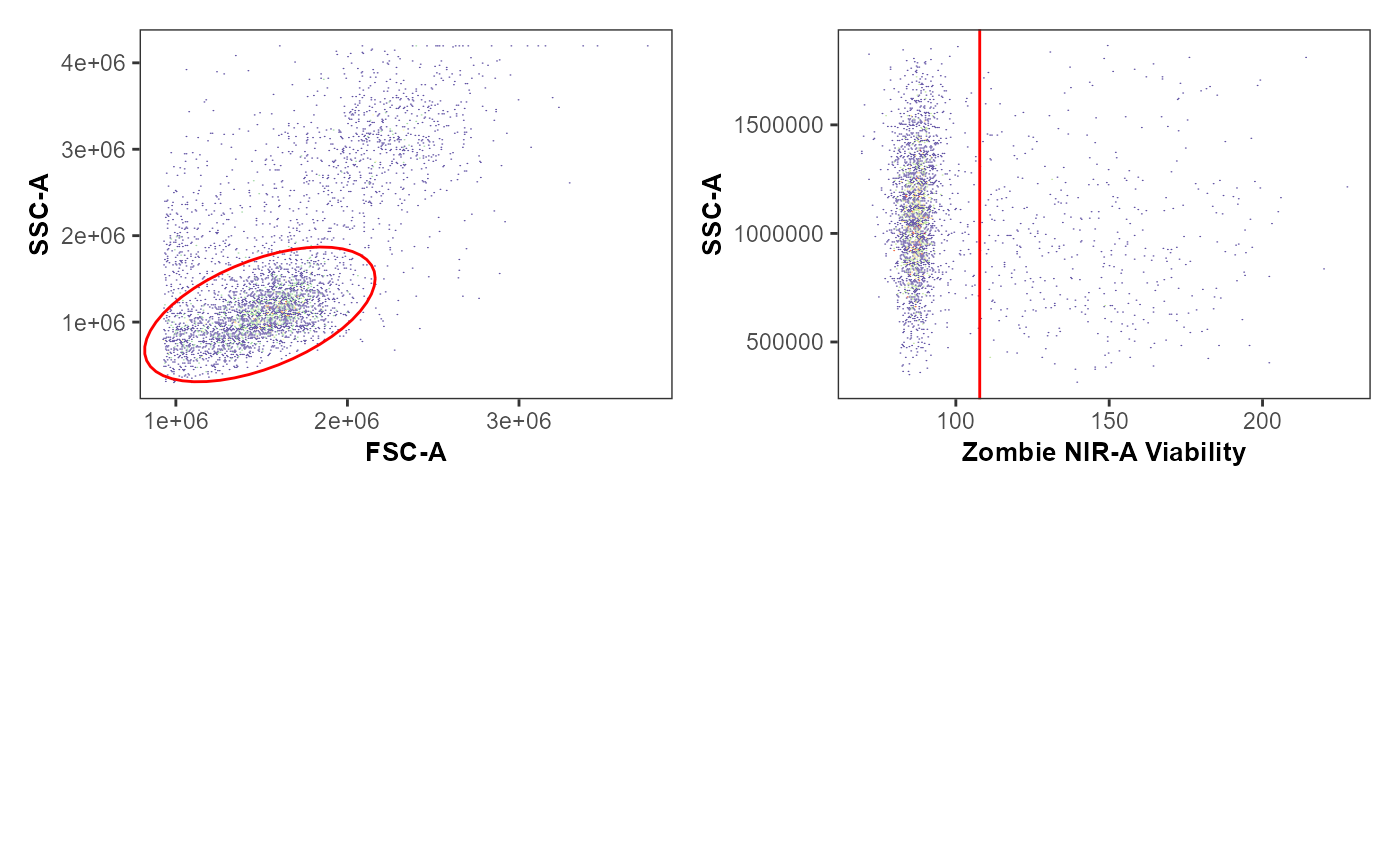 # Visualizing Data
Utility_NxNPlots
Utility_NxNPlots() is a convenient function to visualize
unmixed .fcs files for every marker compared to a reference marker. It
is particularly useful in identifying cell populations, as well as
unmixing errors. It takes a GatingSet object that has been transformed
and gated. The desired population of cells can then be specified by the
gatesubset argument. ycolumn specifies the desired marker to compare all
the other markers to. Similar to other functions that use
Utility_Patchwork behind the scenes, it can send the outputs for each
specimen to their own pdf file.
plot(UnmixedGatingSet)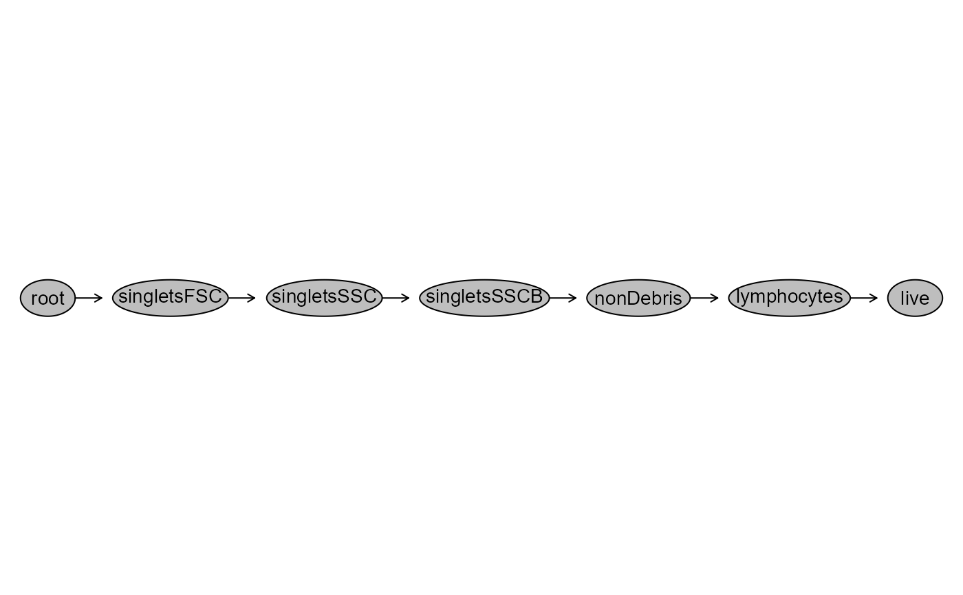
removethese <- c(".fcs", "DTR_")
StorageLocation <- file.path("C:", "Users", "JohnDoe", "Desktop")

colnames(UnmixedGatingSet)[11:39]
#>  [1] "BUV395-A"          "BUV496-A"          "BUV563-A"
#>  [4] "BUV615-A"          "BUV661-A"          "BUV737-A"
#>  [7] "BUV805-A"          "BV421-A"           "Pacific Blue-A"
#> [10] "BV480-A"           "BV510-A"           "BV605-A"
#> [13] "BV650-A"           "BV711-A"           "BV750-A"
#> [16] "BV786-A"           "Alexa Fluor 488-A" "Spark Blue 550-A"
#> [19] "PerCP-Cy5.5-A"     "PE-A"              "PE-Dazzle594-A"
#> [22] "PE-Cy5-A"          "PE-Vio770-A"       "APC-A"
#> [25] "Alexa Fluor 647-A" "APC-R700-A"        "Zombie NIR-A"
#> [28] "APC-Fire 750-A"    "APC-Fire 810-A"

IndividualNxN <- Utility_NbyNPlots(x=UnmixedGatingSet[[4]],
                                   sample.name = "GROUPNAME",
                                   removestrings = removethese,
                                   marginsubset = "lymphocytes",
                                   gatesubset = "live",
                                   ycolumn = "Spark Blue 550-A",
                                   bins = 70, clearance = 0.2,
                                   gatelines = FALSE, reference = NULL,
                                   outpath = StorageLocation,
                                   returntype="patchwork")

MultipleNxN <- map(.x = UnmixedGatingSet[1:2], .f = Utility_NbyNPlots,
                   sample.name = "GROUPNAME", removestrings = removethese,
                   marginsubset = "lymphocytes", gatesubset = "live",
                   ycolumn = "Spark Blue 550-A", bins = 70, clearance = 0.2,
                   gatelines = FALSE, reference = NULL,
                   outpath = StorageLocation, returntype="patchwork")
#> $`1`
The return is for a given specimen all markers vs. the specified
marker on the y-axis. Utility_NxNPlots() additionally
accepts a ycolumn = “ALL” option that will directly iterate over every
marker as the ycolumn argument. However, be warned, for larger SFC
panels with many fluorophores, it will take time for a single specimen
(and each marker pdf taking up memory space!), and even more so over
every specimen in a GatingSet!!!
removethese <- c(".fcs", "DTR_")
StorageLocation <- file.path("C:", "Users", "JohnDoe", "Desktop")

All_IndividualNxN <- Utility_NbyNPlots(x=UnmixedGatingSet[[1]],
                                       sample.name = "GROUPNAME",
                                       removestrings = removethese,
                                       marginsubset = "lymphocytes",
                                       gatesubset = "live", ycolumn = "ALL",
                                       bins = 120, clearance = 0.2,
                                       gatelines = FALSE, reference = NULL,
                                       outpath = StorageLocation,
                                       returntype="pdf")

ALL_MultipleNxN <- map(.x = UnmixedGatingSet, .f = Utility_NbyNPlots,
                       sample.name = "GROUPNAME", removestrings = removethese,
                       marginsubset = "lymphocytes", gatesubset = "live",
                       ycolumn = "ALL", bins = 120, clearance = 0.2,
                       gatelines = FALSE, reference = NULL,
                       outpath = StorageLocation, returntype="pdf")
Utility_ParallelNxNPlots
Utitlity_ParallelNxNPlots is an extension of
Utility_NxNPlots, but is used to compare two separate
samples that are overlaid on the same plot. This can be useful when
comparing different specimens, different treatment conditions, and
differences in unmixing. It is usable but remains under development
(notice the colors from the different specimens don’t blend well). It
utilizes the purrr
purrr::map2() argument behind the scenes to determine the
order of what specimens are compared to each other.
| name |
|---|
| INF071_Ctrl_Tetramer_Unmixed.fcs |
| INF149_Ctrl_Tetramer_Unmixed.fcs |
| INF179_Ctrl_Tetramer_Unmixed.fcs |
| ND050_15_Ctrl_Tetramer_Unmixed.fcs |
OverlaidNxNPlots <- Utility_ParallelNbyNPlots(x=UnmixedGatingSet[1],
                                              y = UnmixedGatingSet[4],
                                              sample.name = "GROUPNAME",
                                              removestrings = ".fcs",
                                              Override = FALSE,
                                              marginsubset = "lymphocytes",
                                              gatesubset = "live",
                                              ycolumn = "Spark Blue 550-A",
                                              bins = 120, clearance = 0.2,
                                              colorX = "lightblue",
                                              colorY = "orange",
                                              gatelines = FALSE,
                                              reference = NULL,
                                              outpath = StorageLocation,
                                              pdf = FALSE)
#> $`1`
Similar to Utility_NxNPlots(), switching the argument
ycolumn = “ALL” will iterate over all marker combinations for y-column
vs all x-marker combinations. The same warning about run time and memory
space applies, but double it as we are overlaying plots.
#Currently bugged out for All Option

gt(pData(UnmixedGatingSet))

All_OverlaidNxNPlots <- Utility_ParallelNbyNPlots(x=UnmixedGatingSet[1],
                                                  y = UnmixedGatingSet[2],
                                                  sample.name = "GROUPNAME",
                                                  removestrings = ".fcs",
                                                  Override = FALSE,
                                                  marginsubset = "lymphocytes",
                                                  gatesubset = "live",
                                                  ycolumn = "ALL", bins = 120,
                                                  clearance = 0.2,
                                                  colorX = "lightblue",
                                                  colorY = "orange",
                                                  gatelines = FALSE,
                                                  reference = NULL,
                                                  outpath = StorageLocation,
                                                  pdf = FALSE)

All_OverlaidNxNPlots[1]
Utility_UnityPlots
While Utility_NxNPlots() will show all marker
combinations for a single specimen, Utility_UnityPlots()
will showcase a single combination of markers for all specimens present
in the GatingSet. Given that bringing data from every specimen into
active memory is a way to max out your ram, it is helpful to break the
map calls into chunks. Here is an example:
SingleUnityPlot <- Utility_UnityPlot(x="Spark Blue 550-A", y="BUV805-A",
                                     GatingSet=UnmixedGatingSet,
                                     sample.name="GROUPNAME", bins=100,
                                     clearance=0.2,removestrings=removestrings,
                                     marginsubset="lymphocytes",
                                     gatesubset="live", gatelines=FALSE,
                                     reference=NULL, returntype="patchwork",
                                     outpath=StorageLocation)
SingleUnityPlot
#> $`1`
Markers <- colnames(UnmixedCytoSet)
KeptMarkers <- Markers[-grep("Time|FS|SC|SS|Original|-W$|-H$|AF", Markers)]
KeptMarkers
#>  [1] "BUV395-A"          "BUV496-A"          "BUV563-A"
#>  [4] "BUV615-A"          "BUV661-A"          "BUV737-A"
#>  [7] "BUV805-A"          "BV421-A"           "Pacific Blue-A"
#> [10] "BV480-A"           "BV510-A"           "BV605-A"
#> [13] "BV650-A"           "BV711-A"           "BV750-A"
#> [16] "BV786-A"           "Alexa Fluor 488-A" "Spark Blue 550-A"
#> [19] "PerCP-Cy5.5-A"     "PE-A"              "PE-Dazzle594-A"
#> [22] "PE-Cy5-A"          "PE-Vio770-A"       "APC-A"
#> [25] "Alexa Fluor 647-A" "APC-R700-A"        "Zombie NIR-A"
#> [28] "APC-Fire 750-A"    "APC-Fire 810-A"
MultipleUnityPlots <- map(.x=KeptMarkers[c(1:6, 8:10)], .f=Utility_UnityPlot,
                          y="BUV805-A", GatingSet=UnmixedGatingSet,
                          sample.name="GROUPNAME", bins=100,clearance=0.2,
                          removestrings=removestrings, marginsubset="lymphocytes",
                          gatesubset="live", gatelines=FALSE, reference=NULL,
                          returntype="patchwork", outpath=StorageLocation)
#> [[1]]
#> [[1]]$`1`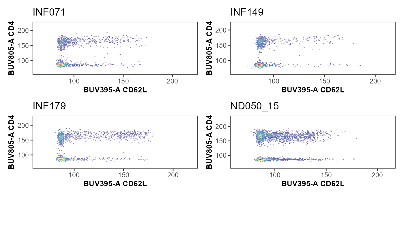
#>
#>
#> [[2]]
#> [[2]]$`1`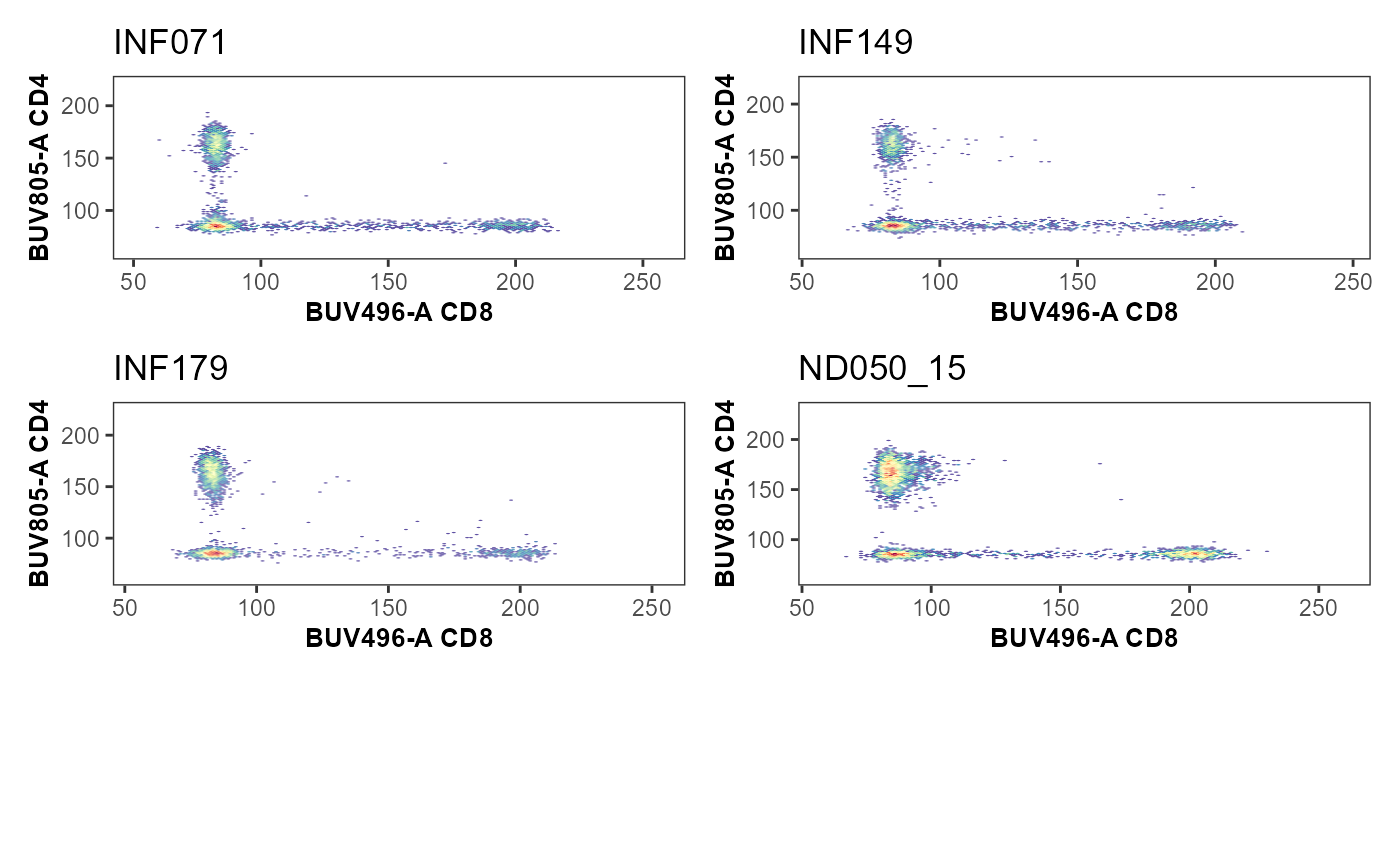
Utility_ThirdColor
Similar to the other visualization functions,
Utility_ThirdColor() plots the data from the specified
GatingSet and subset for the given X and Y axis-markers. From here it
will overlay a color for an additional marker, allowing for
identification of those cells.
Utility_ThirdColor() has three plotting modes that are
called within the splitpoint argument. When “Continuous” is specified,
it takes two colors and forms a color gradient from the lowest to
highest values specified for the parameter specified in the zaxis
argument.
SinglePlot <-  Utility_ThirdColorPlots(x=UnmixedGatingSet[1], subset = "live",
                                       xaxis="BUV496-A", yaxis = "Spark Blue 550-A",
                                       zaxis ="BUV805-A", splitpoint = "continuous",
                                       sample.name = "GROUPNAME",
                                       removestrings = c("DTR", ".fcs"),
                                       thecolor = "blue")
#> Splitpoint is a continuous

AllPlot <- map(.x=UnmixedGatingSet, .f=Utility_ThirdColorPlots, subset = "live",
               xaxis="BUV496-A", yaxis = "Spark Blue 550-A",  zaxis ="BUV805-A",
               splitpoint = "continuous", sample.name = "GROUPNAME",
               removestrings = c("DTR", ".fcs"), thecolor = "blue")
#> Splitpoint is a continuous
#> Splitpoint is a continuous
#> Splitpoint is a continuous
#> Splitpoint is a continuous

SinglePlot 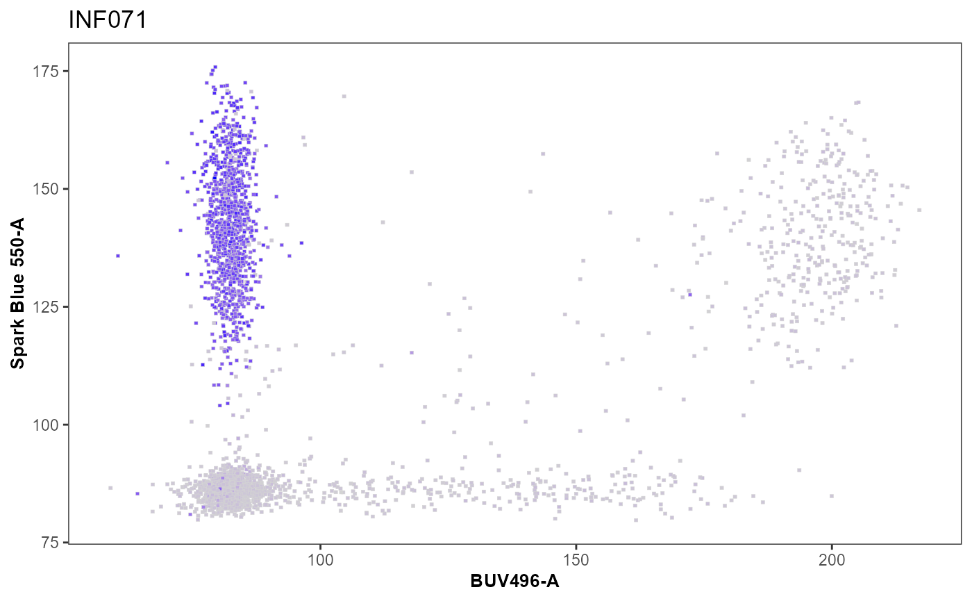
When a categorical column exist in the .fcs file and is specified as zaxis, splitpoint = “Categorical” can be specified. It will internally convert the zaxis column into a factor. A list of equivalent name(s) is then given to FactorNames. These in turn will be filtered and assigned the same color.
ColorTheseFactors <- c("1", "4") #Due to how .fcs files often save factors as numeric values.

SinglePlot <-  Utility_ThirdColorPlots(x=UnmixedGatingSet[1], subset = "live",
                                       xaxis="BUV496-A", yaxis = "Spark Blue 550-A",
                                       zaxis ="BUV805-A", splitpoint = "120",
                                       sample.name = "GROUPNAME",
                                       removestrings = c("DTR", ".fcs"),
                                       FactorNames = ColorTheseFactors,
                                       thecolor = "orange")

AllPlot <- map(.x=UnmixedGatingSet, .f=Utility_ThirdColorPlots, subset = "live",
               xaxis="BUV496-A", yaxis = "Spark Blue 550-A",  zaxis ="BUV805-A",
               splitpoint = "130", sample.name = "GROUPNAME",
               removestrings = c("DTR", ".fcs"), FactorNames = ColorTheseFactors,
               thecolor = "orange")

SinglePlot 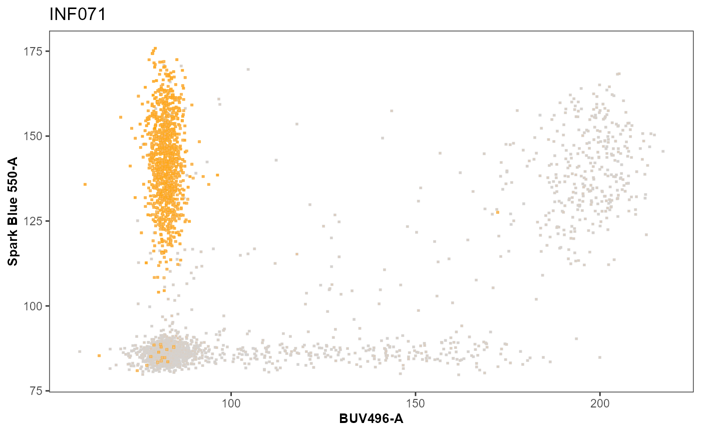
The third option “splitpoint” will dichotomize a continuous marker expression at the given value (either raw MFI or biexponential transformed) into positive and negative cells. It will then shade the cells accordingly.
SinglePlot <-  Utility_ThirdColorPlots(x=UnmixedGatingSet[1], subset = "live",
                                       xaxis="BUV496-A", yaxis = "Spark Blue 550-A",
                                       zaxis ="BUV805-A", splitpoint = "120",
                                       sample.name = "GROUPNAME",
                                       removestrings = c("DTR", ".fcs"),
                                       thecolor = "orange")

SinglePlot 
AllPlot <- map(.x=UnmixedGatingSet, .f=Utility_ThirdColorPlots, subset = "live",
               xaxis="BUV496-A", yaxis = "Spark Blue 550-A",  zaxis ="BUV805-A",
               splitpoint = "130", sample.name = "GROUPNAME",
               removestrings = c("DTR", ".fcs"), thecolor = "orange")
To provide multiple filtering arguments to
Utility_ThirdColorPlots(), a data.frame can be provided to
the splitpoint argument. This is composed of two columns, “Fluorophore”
and “Splitpoint”, with the specified arguments present in the rows. When
a data.frame is detected, Utility_ThirdColorPlots() will
then iterate down the rows to find each gating argument, returning only
the remaining cells that are greater than values listed for each
marker.
FileLocation <- system.file("extdata", package = "Luciernaga")
CSVLocation <- file.path(path = FileLocation, pattern = 'ThirdColorDataFrame.csv')
ThirdColorArguments <- read.csv(CSVLocation)
gt(ThirdColorArguments)| Fluorophore | Splitpoint |
|---|---|
| BUV805-A | 100 |
| BV480-A | 95 |
| PE-Cy5-A | 120 |
SinglePlot <-  Utility_ThirdColorPlots(x=UnmixedGatingSet[1], subset = "live",
                                       xaxis="BUV496-A", yaxis = "Spark Blue 550-A",
                                       zaxis =NULL, splitpoint = ThirdColorArguments,
                                       sample.name = "GROUPNAME",
                                       removestrings = c("DTR", ".fcs"),
                                       thecolor = "orange")
#> Splitpoint is a Dataframe

MultiplePlot <- map(.x=UnmixedGatingSet, .f=Utility_ThirdColorPlots, subset = "live",
                    xaxis="BUV496-A", yaxis = "Spark Blue 550-A",  zaxis =NULL,
                    splitpoint = ThirdColorArguments, sample.name = "GROUPNAME",
                    removestrings = c("DTR", ".fcs"), thecolor = "orange")
#> Splitpoint is a Dataframe
#> Splitpoint is a Dataframe
#> Splitpoint is a Dataframe
#> Splitpoint is a Dataframe

SinglePlot
Utility_ThirdColorPlots can also be used in combination with the Coereba packages GatingCutoff estimates to allow for specimen specific split-points for the specified markers, using the GatingCutoff csv file. This is particularly useful for non-normalized specimens where batch effects are present.
To provide flexibility for your own analysis,
Utility_ThirdColorPlots() returns ggplot objects. These in
turn can be edited, or a list of them passed to and arranged using
Utility_Patchwork() into a .pdf of desired layout.
Utility_DensityOverlay
The function Utility_DensityOverlay() is a wrapper
function incorporating elements from the underlying ggplot2
geom_density() function. It’s use is particularly useful
when working with a GatingSet of multiple specimens and comparing across
individuals.
To use both Utility_DensityOverlay() and
Utility_RidgePlots() to their fullest extent, we will need
to create additional factor variables for each specimen and append them
to the GatingSet’s pData. These can then be called to use as axis, color
and fill arguments for the function. Below you can find examples of
local functions that you can edit for your particular data to extract
variables of interest to append to the pData.
Metadata <- pData(UnmixedGatingSet)
Metadata
#>                                                                  name
#> INF071_Ctrl_Tetramer_Unmixed.fcs     INF071_Ctrl_Tetramer_Unmixed.fcs
#> INF149_Ctrl_Tetramer_Unmixed.fcs     INF149_Ctrl_Tetramer_Unmixed.fcs
#> INF179_Ctrl_Tetramer_Unmixed.fcs     INF179_Ctrl_Tetramer_Unmixed.fcs
#> ND050_15_Ctrl_Tetramer_Unmixed.fcs ND050_15_Ctrl_Tetramer_Unmixed.fcs

NameYoink <- function(x){
pattern <- "(INF|ND)\\d{3}"
result <- stringr::str_extract(x, pattern)
result <- data.frame(result)
colnames(result)[1] <- "specimen"
result$specimen <- factor(result$specimen)
return(result)
}

ConditionYoink <- function(x){
pattern <- "Ctrl|PMA"
result <- stringr::str_extract(x, pattern)
result <- data.frame(result)
colnames(result)[1] <- "condition"
result$condition <- factor(result$condition)
return(result)
}

NormalizedYoink <- function(x){
result <- stringr::str_detect(x, "Norm")
result <- data.frame(result)
colnames(result)[1] <- "normalized"
result$normalized <- factor(result$normalized)
return(result)
}
pd <- pData(UnmixedGatingSet)
pa <- pd %>% select(`name`) %>% pull()
Specimen <- map(pa, .f=NameYoink) %>% bind_rows()
Specimen
#>   specimen
#> 1   INF071
#> 2   INF149
#> 3   INF179
#> 4    ND050
Condition <- map(pa, .f=ConditionYoink) %>% bind_rows
Condition
#>   condition
#> 1      Ctrl
#> 2      Ctrl
#> 3      Ctrl
#> 4      Ctrl
And once we have the factor variables that we need, we can bind the columns together, and then assign them back to the GatingSet.
pd <- cbind(pd, Specimen, Condition)
pData(UnmixedGatingSet) <- pd
pData(UnmixedGatingSet)
#>                                                                  name specimen
#> INF071_Ctrl_Tetramer_Unmixed.fcs     INF071_Ctrl_Tetramer_Unmixed.fcs   INF071
#> INF149_Ctrl_Tetramer_Unmixed.fcs     INF149_Ctrl_Tetramer_Unmixed.fcs   INF149
#> INF179_Ctrl_Tetramer_Unmixed.fcs     INF179_Ctrl_Tetramer_Unmixed.fcs   INF179
#> ND050_15_Ctrl_Tetramer_Unmixed.fcs ND050_15_Ctrl_Tetramer_Unmixed.fcs    ND050
#>                                    condition
#> INF071_Ctrl_Tetramer_Unmixed.fcs        Ctrl
#> INF149_Ctrl_Tetramer_Unmixed.fcs        Ctrl
#> INF179_Ctrl_Tetramer_Unmixed.fcs        Ctrl
#> ND050_15_Ctrl_Tetramer_Unmixed.fcs      Ctrl
StorageLocation <- file.path("C:", "Users", "JohnDoe", "Desktop")

pData(UnmixedGatingSet)
#>                                                                  name specimen
#> INF071_Ctrl_Tetramer_Unmixed.fcs     INF071_Ctrl_Tetramer_Unmixed.fcs   INF071
#> INF149_Ctrl_Tetramer_Unmixed.fcs     INF149_Ctrl_Tetramer_Unmixed.fcs   INF149
#> INF179_Ctrl_Tetramer_Unmixed.fcs     INF179_Ctrl_Tetramer_Unmixed.fcs   INF179
#> ND050_15_Ctrl_Tetramer_Unmixed.fcs ND050_15_Ctrl_Tetramer_Unmixed.fcs    ND050
#>                                    condition
#> INF071_Ctrl_Tetramer_Unmixed.fcs        Ctrl
#> INF149_Ctrl_Tetramer_Unmixed.fcs        Ctrl
#> INF179_Ctrl_Tetramer_Unmixed.fcs        Ctrl
#> ND050_15_Ctrl_Tetramer_Unmixed.fcs      Ctrl
#colnames(UnmixedGatingSet)
Plot <- Utility_DensityOverlay(gs=UnmixedGatingSet, subset="lymphocytes", TheX="APC-Fire 810-A",
                               TheFill="specimen", returntype="plots",
                               outpath=StorageLocation, filename="CD4_Expression")

plotly::ggplotly(Plot[[1]])
Utility_RidgePlots
The function Utility_RidgePlots() leverages the
ggplot2 and ggridges packages to evaluate
marker expression across specimens, and provides some additional
functionality compared to Utility_DensityOverlay()
We can generate a specific RidgePlot of interest by providing the
name of a particular fluorophore in TheX argument. Alternatively, we can
leave it out to generate RidgePlots for all markers. As with the other
functions, it uses Utility_Patchwork() and will take the
same arguments for layout.
StorageLocation <- file.path("C:", "Users", "JohnDoe", "Desktop")

pData(UnmixedGatingSet)
#>                                                                  name specimen
#> INF071_Ctrl_Tetramer_Unmixed.fcs     INF071_Ctrl_Tetramer_Unmixed.fcs   INF071
#> INF149_Ctrl_Tetramer_Unmixed.fcs     INF149_Ctrl_Tetramer_Unmixed.fcs   INF149
#> INF179_Ctrl_Tetramer_Unmixed.fcs     INF179_Ctrl_Tetramer_Unmixed.fcs   INF179
#> ND050_15_Ctrl_Tetramer_Unmixed.fcs ND050_15_Ctrl_Tetramer_Unmixed.fcs    ND050
#>                                    condition
#> INF071_Ctrl_Tetramer_Unmixed.fcs        Ctrl
#> INF149_Ctrl_Tetramer_Unmixed.fcs        Ctrl
#> INF179_Ctrl_Tetramer_Unmixed.fcs        Ctrl
#> ND050_15_Ctrl_Tetramer_Unmixed.fcs      Ctrl
#colnames(UnmixedGatingSet)

SinglePlot <- Utility_RidgePlots(gs=UnmixedGatingSet, subset="live", TheFill="condition",
                           TheX = "APC-Fire 810-A", TheY="specimen", returntype="plots",
                           outpath=StorageLocation, filename="RidgePlot_Condition")

SinglePlot[[1]]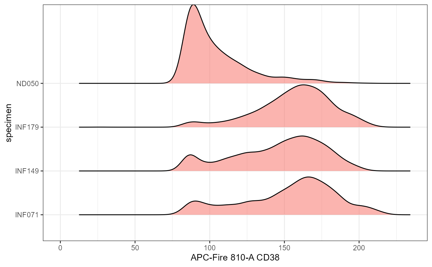
Plot <- Utility_RidgePlots(gs=UnmixedGatingSet, subset="live", TheFill="condition",
                           TheY="specimen", returntype="patchwork",
                           outpath=StorageLocation, filename="RidgePlot_Condition")
Plot[1:2]
#> $`1`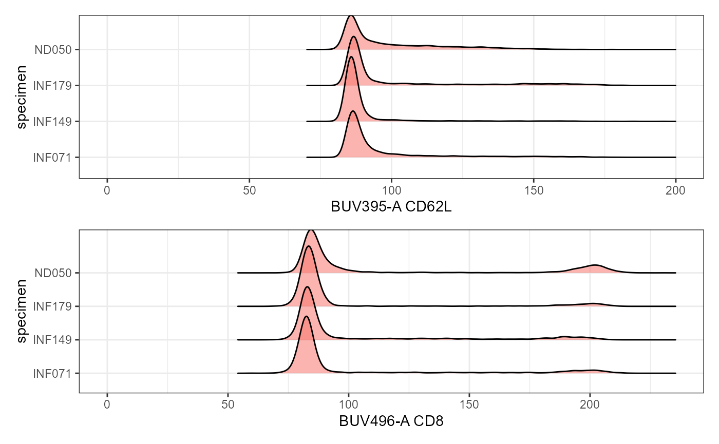
#>
#> $`2`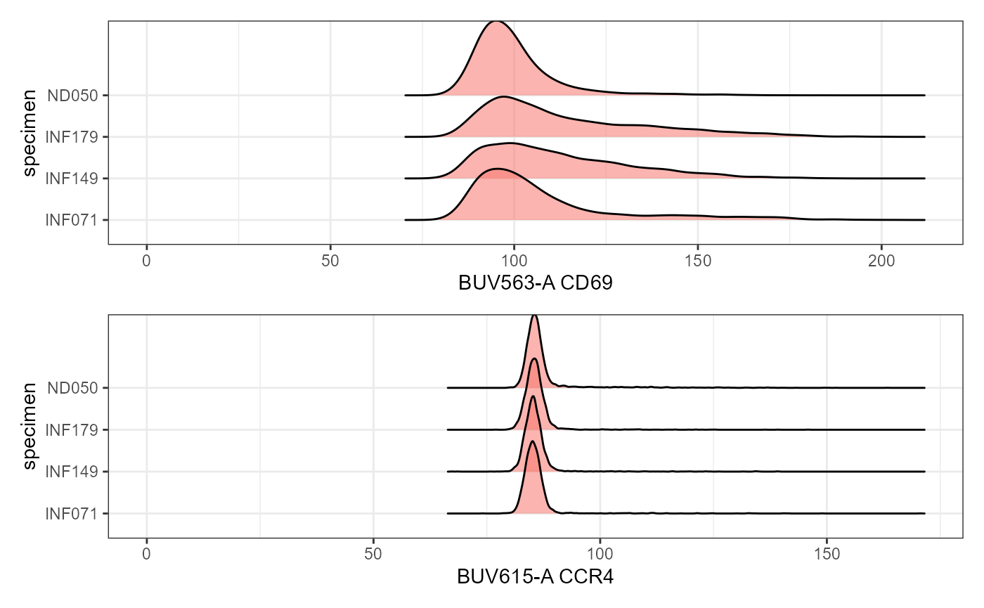
Future Development
In combination with purrr package functions, it’s possible to extend the visualization capacity for many scenarios similar to Utility_UnityPlots and Utility_NxNPlots. As community usefulness is demonstrated, these will become integrated in later versions of the package. Reach out via the GitHub for suggested improvements.
#> R version 4.4.1 (2024-06-14 ucrt)
#> Platform: x86_64-w64-mingw32/x64
#> Running under: Windows 11 x64 (build 26100)
#>
#> Matrix products: default
#>
#>
#> locale:
#> [1] LC_COLLATE=English_United States.utf8
#> [2] LC_CTYPE=English_United States.utf8
#> [3] LC_MONETARY=English_United States.utf8
#> [4] LC_NUMERIC=C
#> [5] LC_TIME=English_United States.utf8
#>
#> time zone: America/New_York
#> tzcode source: internal
#>
#> attached base packages:
#> [1] stats     graphics  grDevices utils     datasets  methods   base
#>
#> other attached packages:
#>  [1] htmltools_0.5.8.1    plotly_4.10.4        gt_0.11.1
#>  [4] stringr_1.5.1        purrr_1.0.2          dplyr_1.1.4
#>  [7] data.table_1.16.2    ggcyto_1.32.0        ncdfFlow_2.50.0
#> [10] BH_1.84.0-0          ggplot2_3.5.1        openCyto_2.16.1
#> [13] flowWorkspace_4.16.0 flowCore_2.16.0      Luciernaga_0.99.2
#> [16] BiocStyle_2.32.1
#>
#> loaded via a namespace (and not attached):
#>  [1] tidyselect_1.2.1    viridisLite_0.4.2   farver_2.1.2
#>  [4] viridis_0.6.5       fastmap_1.2.0       lazyeval_0.2.2
#>  [7] XML_3.99-0.17       digest_0.6.37       timechange_0.3.0
#> [10] lifecycle_1.0.4     magrittr_2.0.3      compiler_4.4.1
#> [13] rlang_1.1.4         sass_0.4.9          tools_4.4.1
#> [16] utf8_1.2.4          yaml_2.3.10         figpatch_0.2
#> [19] knitr_1.48          labeling_0.4.3      htmlwidgets_1.6.4
#> [22] plyr_1.8.9          xml2_1.3.6          RColorBrewer_1.1-3
#> [25] Rtsne_0.17          withr_3.0.1         RProtoBufLib_2.16.0
#> [28] BiocGenerics_0.50.0 desc_1.4.3          grid_4.4.1
#> [31] stats4_4.4.1        fansi_1.0.6         colorspace_2.1-1
#> [34] progressr_0.15.1    scales_1.3.0        ggridges_0.5.6
#> [37] cli_3.6.3           rmarkdown_2.28      ragg_1.3.3
#> [40] generics_0.1.3      rstudioapi_0.17.0   httr_1.4.7
#> [43] reshape2_1.4.4      cachem_1.1.0        zlibbioc_1.50.0
#> [46] parallel_4.4.1      BiocManager_1.30.25 matrixStats_1.4.1
#> [49] vctrs_0.6.5         Matrix_1.7-0        jsonlite_1.8.9
#> [52] lsa_0.73.3          cytolib_2.16.0      bookdown_0.41
#> [55] patchwork_1.3.0     S4Vectors_0.42.1    RBGL_1.80.0
#> [58] Rgraphviz_2.48.0    crosstalk_1.2.1     systemfonts_1.1.0
#> [61] jquerylib_0.1.4     hexbin_1.28.4       tidyr_1.3.1
#> [64] glue_1.8.0          pkgdown_2.1.1       uwot_0.2.2
#> [67] stringi_1.8.4       lubridate_1.9.3     gtable_0.3.5
#> [70] munsell_0.5.1       tibble_3.2.1        pillar_1.9.0
#> [73] graph_1.82.0        R6_2.5.1            textshaping_0.4.0
#> [76] evaluate_1.0.1      lattice_0.22-6      Biobase_2.64.0
#> [79] highr_0.11          SnowballC_0.7.1     bslib_0.8.0
#> [82] Rcpp_1.0.13         flowClust_3.42.0    gridExtra_2.3
#> [85] xfun_0.48           zoo_1.8-12          fs_1.6.4
#> [88] pkgconfig_2.0.3